
The assumption that advertising revenues will grow proportionally to cost is usually unrealistic. The relationship between revenue generated by advertising and its cost is most often nonlinear, and as expenditures increase, we can expect diminishing marginal revenue gains. So how can this function be described?
Why Does Marginal Effectiveness Decrease?
At least after a certain point, we should expect that each additional euro spent on advertising will yield increasingly smaller returns.
The decreasing marginal effectiveness of advertising is due to several factors. One reason is that increasing investment in a given marketing channel involves displacing a larger number of competitors.
Competition in advertising is usually broader than our direct market competition. It includes all companies targeting the same audience and wanting to advertise in the same channels.
This means paying higher click or impression rates, which is especially evident in real-time auctions based advertising systems, such as Meta, Google, and most social media platforms and RTB advertising networks.
A remedy for this could be to include new marketing channels, which would allow reaching new audiences, but as investment grows, there will be increasing overlap of target groups between channels (known as cannibalization).
Finally, increasing frequency of ad impressions and a growing number of consumer touchpoints with advertising leads to a decreased reaction to subsequent ad exposures.
For example, the twentieth impression of an ad is likely to affect the viewer less than its first impression.
There can be more factors contributing to this. All of them are manifestations of a universal economic principle – the law of diminishing returns. This principle states that each additional unit of input yields progressively smaller increments of output.
When creating business models, we would expect the relationship between advertising cost and revenue to be described by a mathematical function, rather than just stating that marginal revenue will decline.
Search Engine Marketing
In search engines, we deal with a limited number of available impressions. The volume of queries related to a specific search term is a result of consumer behaviour, and we cannot increase it by raising CPC rates and spending more on SEM.
If there are, on average, 500 searches for the term “impact drill” per day in a given period, we will not influence this by investing more in ads for that keyword. For each impression, there is a limited number of advertising spots, such as four paid search results at the top of the page and eight visible product ads – and that is essentially all that generates any significant traffic. SEM specialist joke that more people have seen the dark side of the Moon than the second page of Google – and they do it for a reason.
It is therefore evident that at some point, SEM will hit a “ceiling.” Similar mechanisms will, of course, also occur in other advertising media.
In the case of SEM, we will encounter less reduced user response to subsequent ad interactions, as the ads are initiated by the user, who for some reason is (still) searching in Google rather than going to our site.
Search engine campaigns will also provide less deferred effects. SEM is a “direct response” activity, and aside from the typical time lag between interaction and conversion (a longer or shorter decision-making process), it has limited impact on long-term brand awareness.
Therefore, the relationship between the cost and revenue from search engine advertising will be primarily influenced by competition mechanisms among advertisers within the search engine itself.
The cost of advertising will also be influenced by the pricing policies of search engines. While click costs are set in an auction, Google and other search engines use additional mechanisms that allow them to influence CPC.
For example, the first page minimum bid or the top of the page will minimum bid will prevent us fro buying ads for a very low price, even if there is no competition for a given keyword or other advertisers have temporarily exhausted their budgets.
We should assume that Google’s and other search engines’ auction algorithms aim to set CPC at a level where their revenue is maximised, considering current demand and advertisers’ willingness to accept a given price.
Typical Revenue and Cost Relationship in Search Engines
Based on data from Google Ads Performance planner, it is possible to determine how much revenue (conversions) can be obtained from a campaign as the budget increases. An example distribution of values looks like this:
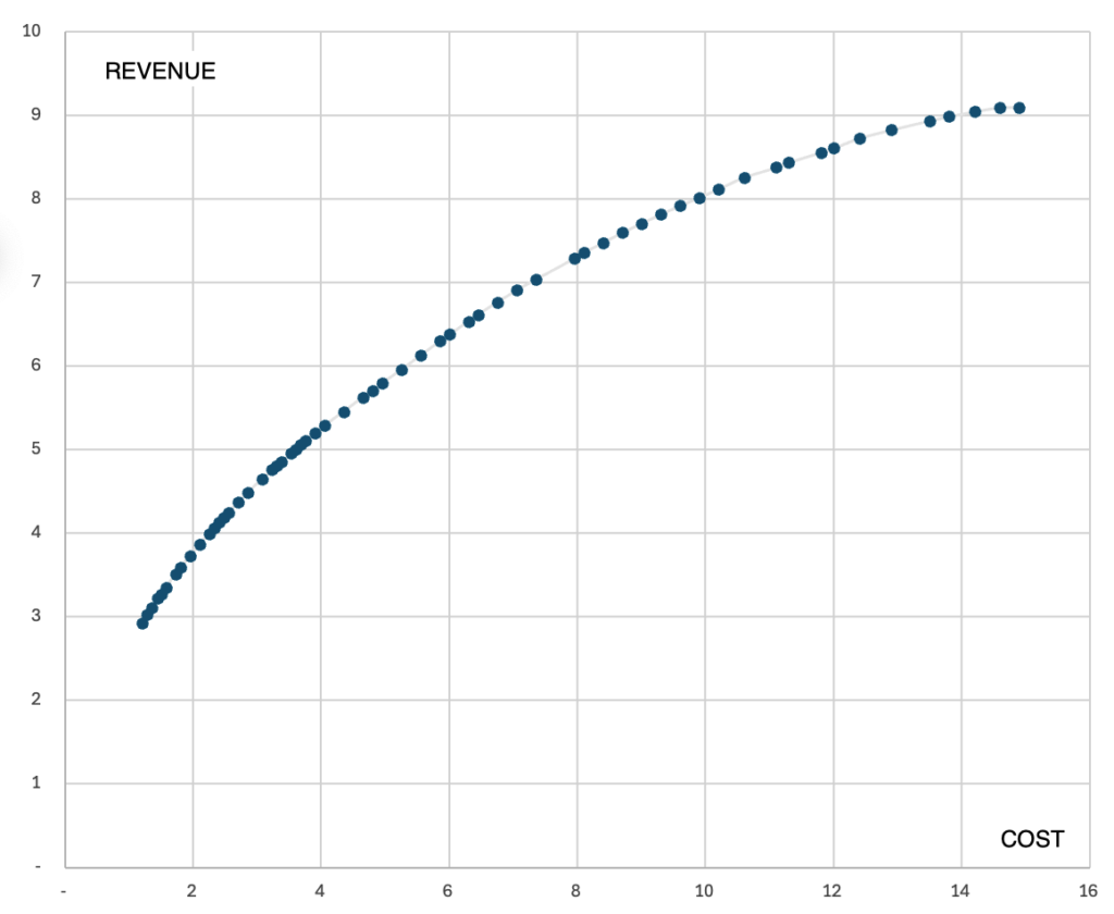
What mathematical function can describe this relationship? This function should:
- Be an increasing function (higher cost mean higher revenues);
- Be a concave function (grow more slowly, causing its graph to curve);
- Have a horizontal asymptote, meaning a maximum value that it will never exceed (each marketing channel has its own “ceiling”);
- For a cost of 0, also have a value of zero.
To identify the mathematical relationship between revenue (R) and cost (C), it is useful to examine the relationships between related parameters and look for (preferably) linear dependencies.
Linearly Increasing ERS as a Function of Revenue (Constant Elasticity)
The most commonly used profitability measure is ROAS (Return On Ad Spend). However, in marginal cost analysis, a more convenient measure is ERS (Effective Revenue Share), which is the mathematical inverse of ROAS:
ERS = C/R = 1/ROAS
Unlike ROAS, the ERS coefficient, like CPC and CPA, increases as campaigns intensify, making it a more intuitive measure of the unit cost of generating revenue.
The relationship between ERS and campaign revenue in this example is as follows:
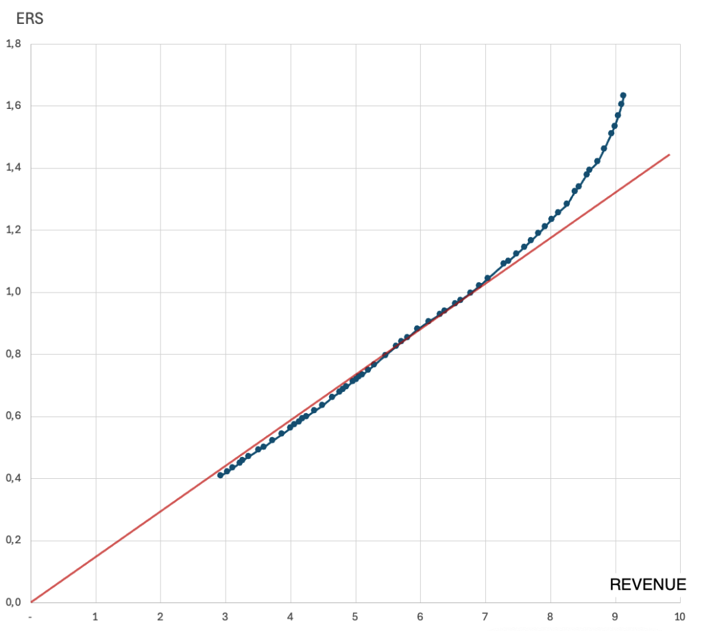
As seen, over a significant range, it is a linear function, which only starts to curve when revenues exceed 7 (million EUR).
A linear relationship between ERS and revenue indicates that the price elasticity of converting traffic in this case is constant. Price elasticity is defined as follows:
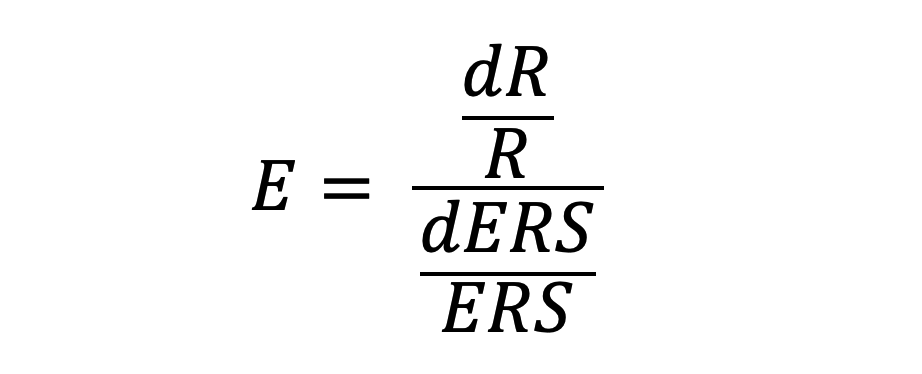
where d represents a very small increment.
It is the ratio of the relative (percentage) increase in revenue to the relative increase in price. Elasticity tells us how quickly generated revenues grow as rates increase and the accepted cost of acquisition rises. In our case, it oscillates around a value of E = 0.94.
Elasticity close to one is frequently encountered in advertising auctions, as it is the value that maximizes search engine profits. The reasons for this phenomenon are described in detail in this article in Search Engine Land.
Assuming elasticity is constant, the function describing the revenue-cost relationship is:
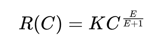
where K is a constant that can be determined from current values. The derivation of this formula can be found here (PDF file).
Here is how this function applied to the discussed simulation looks:
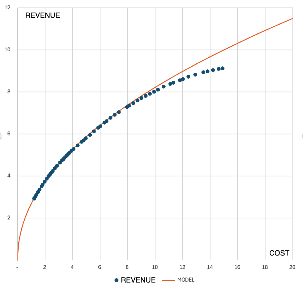
As seen, it very accurately reflects the values from the simulation over a wide range. Discrepancies start to appear after exceeding 8 (million PLN) in costs.
However, this function does not have a horizontal asymptote: for infinite costs, its value will tend towards infinity, so its use will always be limited to a certain range of expenditures.
This also proves that price elasticity cannot be constant and must decrease as cost increase, meaning the drop in effectiveness must accelerate.
Linearly Increasing ERS as a Function of Cost
The relationship between ERS and campaign cost in this example looks like this:
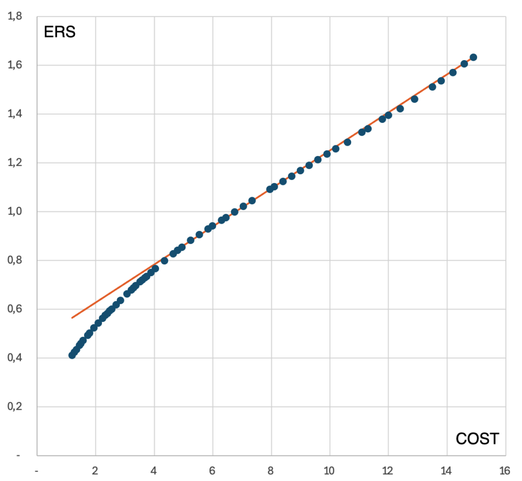
The value distribution is close to linear for costs above 8 (million PLN). If we describe this relationship:
ERS = aC + b
i.e.,
C/R = aC + b
then the function describing the revenue-cost relationship will be:
R(C) = C / (aC + b)
This function (green line) aligns with the simulation values for costs above 8 (million PLN):
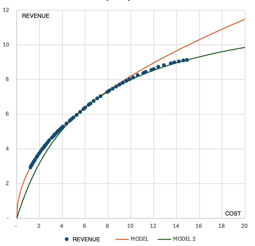
This function (green line) has a horizontal asymptote: its value at infinity tends towards 1/a (in this case, it is 12.8, i.e. according to this simulation, this is the maximum revenue from this campaign, even if we invested an unlimited sum of money).
So, we can write Rmax = 1/a. Let’s now calculate the cost C½ needed to generate half the maximum revenue, Rmax / 2 = 1/(2a), substituting these values into the formula for R(C) and solving the equation:
1/(2a) = C½ / (aC½ + b)
i.e.
C½ = b/a
Therefore, the function R(C) = C / (aC + b) can also be written as:
With the model based on constant elasticity (orange line), these functions allow modeling campaigns over a wide range of revenues and costs.
The Hill Function
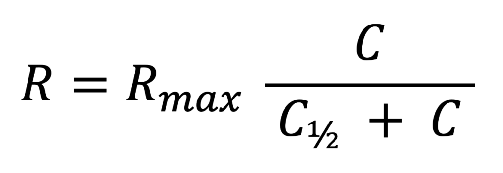
When modeling advertising revenue, the Hill function can also be used. This function, derived from biochemistry, is primarily used to describe physiological processes, such as the binding of oxygen to hemoglobin in the blood or to predict how different toxin concentrations affect organisms.
It turns out that it is well-suited for modeling advertising effectiveness. Its form is:
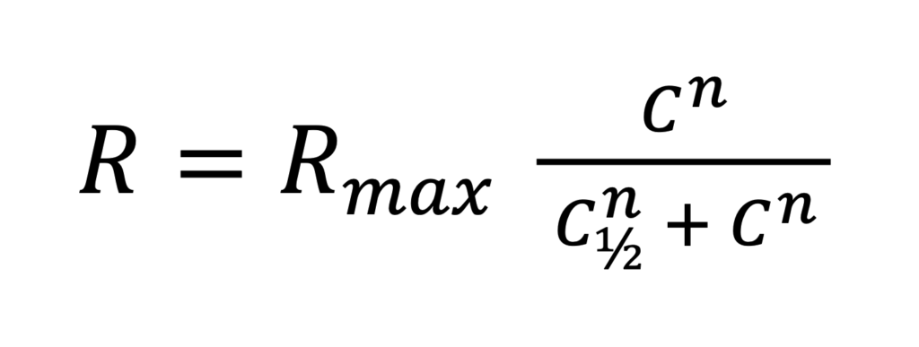
where:
Rmax – the maximum revenue value that can be generated from a given ad (“ceiling”)
C½ – the cost to achieve half of the maximum possible revenue, i.e., the cost value C for which the function R(C) has the value:
R(C½) = 1/2 Rmax
n – a coefficient determining the shape of the function:
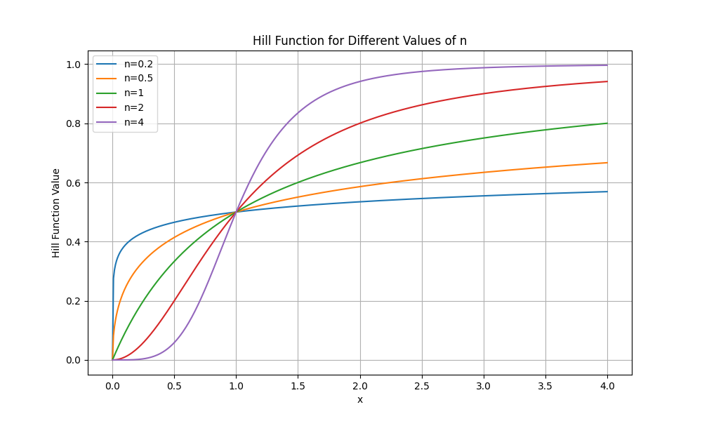
This function meets the assumed conditions: it is increasing, passes through the point (0, 0), has a horizontal asymptote (Rmax), and for n ≤ 1 is a concave function. For n = 1, it yields a model identical to the linear ERS(C) function described earlier.
For the discussed example, the best fit for the Hill function is obtained with Rmax = 23.36, C½ = 29.02, n = 0.62.
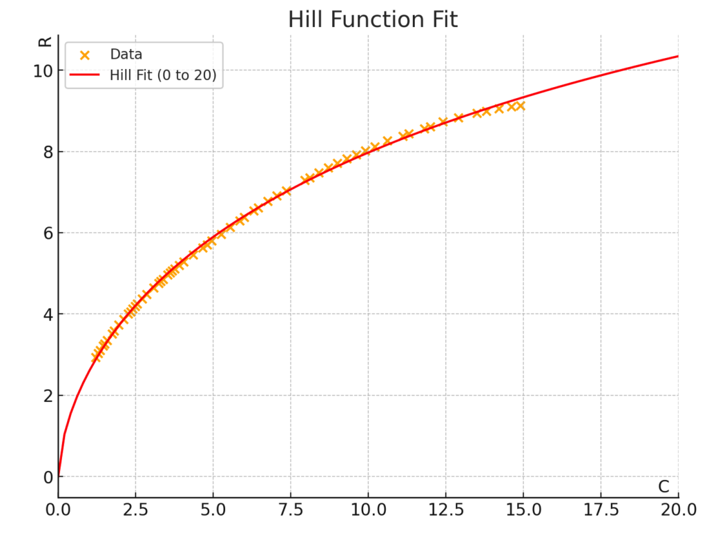
However, the Hill function is not a universal solution for accurately representing every R(C) function. Often, it will be necessary to use a combination of two or more functions for different expenditure ranges (see other examples of R(C) distributions in this PDF file).
Of course, the question remains whether a few percent deviation from the model is a real problem for forecasting with such high uncertainty, as in forecasting advertising results.
You might also be interested in an article on Profit Driven Management of PPC Campaigns.